Handling missing data - Things Solver

Hi, everyone. Although I planned for my next post to be about anomaly detection and their treatment, I faced some other type of problem that quickly escalated into huge issue affecting the modelling and results accuracy, and couldn’t resist to share my experience as soon as possible. In this post, I will be talking about the problem of handling missing data.

Missing data represents an everyday problem for an analyst. We got used to it, and most often, we just treat it with some standard techniques, and continue with the analysis. That’s what I’ve done, until I realized it’s not giving satisfying results.

We’ve all been taught that the easiest way of handling missing values is to drop them, of course, if there’s not too many of it. If there is a significant number of missing values, some other options include filling it with some value. The trickiest part here is deciding how those missing values should be filled.

Before making this decision, it is important to know that there are three types of data missingness, and it is not a shame if you haven’t yet heard of it – I must admit that I recently found it out.

The possible types of missing data are:

1. Missing completely at random (MCAR) – the occurrence of missing values for a variable is not related to the missing value, the values of other variables or the pattern of missingness of other variables (systematic missingness, resources constraints, regime censure);

2. Missing at random (MAR) – the occurrence of missing values for a variable is random, contingent on the value or the missingness of observable variables (contained poll answers, faulty measures, etc);

3. Missing not a random (MNAR) – the occurrence of the missing values is systematically related to unknown or unmeasured covariate factors (we don’t know how it happens and thus cannot model it in any way).

The most important thing to notice here is that the third type of missingness is untreatable. The good news are – the other two are. So, if the type of the missingness is MCAR or MAR, but the data is not modelled, the whole process would result in low efficiency, and in latter case – bias. The conclusion is – we should model it somehow, and we will get to it. But first, let’s list treatment techniques.

1. Dropping instances with missing values – as mentioned above, it would result in low efficiency problem, and could even bias in the case of MAR. But let’s look at the example below. This technique would delete both instances, which will be a huge loss of information if there are many instances like the one with ID=1.

ID	x	y	z	w
1	2.50	0.18	10.50	–
2	–	–	–	–

2. Mean imputation – the mean value of observed values is calculated for each variable, and missing values for that variable are filled with it. In the example below, we would fill the missing value for variable w with the value of 37, when actually it should be 49. If it was the age, it is quite a difference, and in practice, it would be even worse.

ID	x	y	z	w
1	2.50	0.18	10.50	55
2	2.70	0.23	11.75	–
…	…	…	…	…
3	1.50	0.12	12.80	19

3. Regression-based imputation – in this case, it is assumed that, for example, w could be calculated as a linear combination of other variables for a given instance, and that is pretty awesome if there is noticeable correlation between variables. So, for the example above, it could be noticed that when x and y are higher, the w is higher, and when they are lower, the w is also low. Analogically, it is noticeable that there is the negative correlation between y and w. So, here would the calculated value of 48 be more convenient.

4. Data interpolation – it is used in time series mostly, when the missing value could be filled with the value from the previous time period, or with the average of two neighbor time period values.

5. Multiple imputation – in this case, the imputation is performed multiple times, for each variable that is missing, using independent as well as dependent variables. One of the most used algorithms with this kind of logic is the MICE algorithm, and we will be talking about it below.

Multiple imputation using chained equations a.k.a. MICE

MICE algorithm is used when facing a problem of MAR missing data – data that is missing at random but dependent on observable variables. It is generally consisted of these steps:

1. Imputation of means – every missing value for a particular variable is replaced with the mean value for that variable;

2. At this step, one variable is selected and its filled missing values are set back to null;

3. A regression model is run for observed values of the variable from step 2. In this regression model, variable from the second step is used as dependent, while (some or all) other variables are used as independent;

4. The missing values for variable from step 2 are then replaced with regressed values obtained from applying the trained model;

5. Steps 2-4 are then applied for every variable in the dataset. Iterating through each of these variables constitutes one cycle. At the end of one cycle, all of the missing values have been replaced with predictions from regressions that reflect the relationships observed in the data;

6. Steps 2-4 are repeated for a number of cycles, usually ten. It is expected that regression coefficients would converge by the n-th cycle, and the result is a complete dataset.

Easy logic, and what’s more important, I came up to such a nice implementation that makes the use of this algorithm even easier. The library is called fancyimpute and you can find the library and docs here. As usually, I’m not gonna bother you much with the code, you can find it in the link, and it’s really two lines of code.

I tested this library in two ways. First, I ran it for the object whose features were fully filled. I randomly set some values to null, and then ran the model. After this, I calculated the RMSE between the imputed and real values, and RMSE was pretty satisfying.

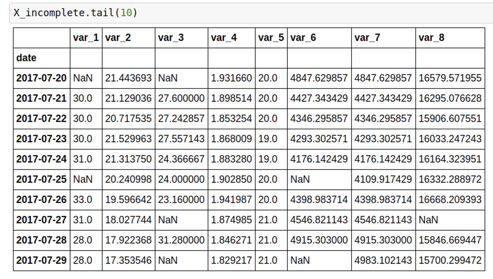
My test dataset looked like this.

Here’s the code.

# import the library
from fancyimpute import  MICE

# convert dataframe to matrix, to make it workable with
X_incomplete_matrix = X_incomplete.as_matrix()

# call the function to impute the values
X_filled_mice = MICE(min_value=0).complete(X_incomplete_matrix)

# make a dataframe out of results
X_complete_with_mice = pd.DataFrame(X_filled_mice, columns = X_complete.columns)

It was easy to compare the results with X_complete, that contained real values. You can see the goodness of fit below.

Of course, the RMSE depends on the number of missing values, the more missing values – the higher the error. That’s why we derived one additional feature for every instance that would help us working with dataset, interpreting results and making decisions, called “confidence”. Confidence equal to 100 means the instance has values for all the features, and it is decreasing as the number of missing values increases.

The second way of validation included consultations with the domain expert and his word of approval. We concluded that the missing values were pretty accurately imputed, so we could continue with the analysis normally.

I will investigate other methods of handling missing values more in the future, and will share my experiences here. I would be happy to hear that someone has also tried this, or any of the other algorithms implemented in the above mentioned library. Of course, if you have any questions, please, do not hesitate to comment below, I’ll do my best to answer it clearly and as soon as possible.