
In the previous text, we talked about the basics of streaming, what it means in theory, what are the advantages, disadvantages and mentioned some streaming tools.
This text is more technical, and we will talk about Flink in general as well as the basics of streaming in Flink, the whole process from start (read data) to end (write streaming results), using the Python API, with a little help from Kafka. The use-case is very simple, with only seven parameters per event, but what is important is that you will be able to easily expand the use-case by yourself if you understand how everything below works. Although the title states with “banking”, it can be applied in any industry, of course.
What is Apache Flink?

Apache Flink is an open-source framework used for distributed data-processing at scale. Flink is primarily used as a streaming engine but can be used as well as a batch processing engine. The initial release was 9 years ago and it’s developed in Java and Scala. Alongside those two languages, Python API is available as well, and that’s the one we are going to use in this example. Flink integrates with all common cluster resource managers such as Hadoop YARN, Apache Mesos, and Kubernetes but can also be set up to run as a stand-alone cluster.
Flink provides an extremely simple high-level API in the form of Map/Reduce, Filters, Window, GroupBy, Sort and Joins. Talking about the advantages for Flink, we should not forget the main advantage of streaming compared to batch processing and that’s minimal resources. Exactly, Flink provides you that. In terms of development, also support SQL in queries which can be of great benefit to people with less technical knowledge.
Sources and sinks can be retrieved from various sources:
- Filesystem (source/sink)
- Apache Kafka (source/sink)
- Apache Cassandra (sink)
- Amazon Kinesis Streams (source/sink)
- Elasticsearch (sink)
- Hadoop FileSystem (sink)
- RabbitMQ (source/sink)
- Apache NiFi (source/sink)
- Twitter Streaming API (source)
- Google PubSub (source/sink)
- JDBC (sink)
Basic PyFlink use-case
After a small introduction to Apache Flink, let’s get hands on the real example with code. This example consists of a python script that generates dummy data and loads it into a Kafka topic. Flink source is connected to that Kafka topic and loads data in micro-batches to aggregate them in a streaming way and satisfying records are written to the filesystem (CSV files).
Step 1 – Setup Apache Kafka
Requirements za Flink job:
Kafka 2.13-2.6.0
Python 2.7+ or 3.4+
Docker (let’s assume you are familiar with Docker basics)
Our test project has this structure:
streaming_with_kafka_and_pyflink
  - docker-pyflink
    - image
       Dockerfile
    - examples
      - data
        - output
          - output_file.csv
      - app
        app.py
    - docker-compose.yml
  - data-generators
    - dummy_data_generator.py
So, let’s start with this mini use case flow.
First of all, get Kafka from here:
Then tar that file with:
tar -xzf kafka_2.13-2.6.0.tgz
cd kafka_2.13-2.6.0
Add code blocks below to serve.properties to ensure Flink in Docker can see Kafka topics running locally:
listeners=EXTERNAL://0.0.0.0:19092,INTERNAL://0.0.0.0:9092
listener.security.protocol.map=INTERNAL:PLAINTEXT,EXTERNAL:PLAINTEXT
advertised.listeners=INTERNAL://127.0.0.1:9092,EXTERNAL://docker.for.mac.localhost:19092
inter.broker.listener.name=INTERNAL
To the end of config/server.properties file and then run Zookeeper and Kafka:
bin/zookeeper-server-start.sh config/zookeeper.properties
bin/kafka-server-start.sh config/server.properties
Now your Kafka is ready. One thing that is left is to create a Kafka topic that will be used in this case, let’s call it “transactions-data”.
bin/kafka-topics.sh --create --zookeeper localhost:2181 --replication-factor 1 --partitions 1 --topic transactions-dataStep 2 – Create a dummy data
Of course, having data is the biggest requirement of all. For those who have already predefined data for the test, please skip this step. But if you don’t, follow instructions for the Python script we are using to create dummy data. In addition to other libraries, we are using library Faker to create fake user names. So, there is no real person in this example.
Let’s take a look at the python script for generating dummy data:
On the top is the import of necessary libraries, some of them you will get immediately with Python installation, the other you should install manually.
import time
import datetime
import random
import pandas as pd
from faker import Faker
from kafka import KafkaProducer
from json import dumps
In the next code-block, you can see functions used for generating random users, spent amount for each user, type of transaction, location and DateTime of the event.
fake = Faker()
start_time = time.time()

list_of_transactions = ['highway_toll', 'petrol_station', 'supermarket', 'shopping',
                        'mortgage', 'city_service', 'restaurant', 'healthcare']

def generate_random_users():
    list_of_users = []
    for number in range(100):
        list_of_users.append(fake.name())
    return list_of_users

def get_random_user(users):
    return random.choice(users)

def get_usage_amount():
    a = [0, round(random.randint(1, 100) * random.random(), 2)]
    random.shuffle(a)
    return a

def get_usage_date():
    return fake.date_time_between(start_date='-1m', end_date='now').isoformat()

def create_usage_record(list_of_users):
    amount = get_usage_amount()
    return {
        'customer': get_random_user(list_of_users),
        'transaction_type': random.choice(list_of_transactions),
        'online_payment_amount': amount[0],
        'in_store_payment_amount': amount[1],
        'transaction_datetime': get_usage_date(),
    }
The third code-block contains the time range we are going to put our script to generate data until we break (and we choose almost 50 years ahead). In that time-range, the script will generate 1000 records with a pause of 5 seconds. All generated data will be sent to a Kafka topic called data_usage.
users = generate_random_users()
end_datetime = datetime.datetime.combine(datetime.date(2070, 1, 1), datetime.time(1, 0, 0))
current_datetime = datetime.datetime.combine(datetime.date.today(), datetime.datetime.now().time())
while current_datetime <= end_datetime:
    data_usage = pd.DataFrame([create_usage_record(users) for _ in range(1000)])
    producer = KafkaProducer(bootstrap_servers=['localhost:9092'],
                             value_serializer=lambda x: dumps(x).encode('utf-8'))

    for row in data_usage.itertuples():
        data_customer = row.customer
        data_transaction_type = row.transaction_type
        data_online_payment_amount = row.online_payment_amount
        data_in_store_payment_amount = row.in_store_payment_amount
        data_lat = random.uniform(44.57, 44.91)
        data_lon = random.uniform(20.20, 20.63)
        data_transaction_datetime = row.transaction_datetime + "Z"
        data = {
                'customer': data_customer,
                'transaction_type': data_transaction_type,
                'online_payment_amount': data_online_payment_amount,
                'in_store_payment_amount': data_in_store_payment_amount,
                'lat': data_lat,
                'lon': data_lon,
                'transaction_datetime': data_transaction_datetime
                }
        future = producer.send('transactions-data', value=data)
        result = future.get(timeout=5)
    print("--- {} seconds ---".format(time.time() - start_time))
    time.sleep(5)
    current_datetime = datetime.datetime.combine(datetime.date.today(), datetime.datetime.now().time())
After Kafka installation, we can start a Python script for generating dummy data and load them into the topic. The last step is to create another Python script. But this time with Flink functions. To avoid differences between operating systems, we packed a script with Flink functions into Docker. That way we are sure it will work on every operating system without any or at least, major changes.
Step 3 – Load data to Flink
In the script below, called app.py we have 3 important steps. Definition of data source, the definition of data output (sink) and aggregate function.
Let’s go step by step. The first of them is to connect to a Kafka topic and define source data mode.
import os
from pyflink.datastream import StreamExecutionEnvironment, TimeCharacteristic
from pyflink.table import StreamTableEnvironment, CsvTableSink, DataTypes, EnvironmentSettings
from pyflink.table.descriptors import Schema, Rowtime, Json, Kafka, Elasticsearch
from pyflink.table.window import Tumble
 def register_transactions_source(st_env):
    st_env.connect(Kafka()
                   .version("universal")
                   .topic("transactions-data")
                   .start_from_latest()
                   .property("zookeeper.connect", "host.docker.internal:2181")
                   .property("bootstrap.servers", "host.docker.internal:19092")) \
        .with_format(Json()
        .fail_on_missing_field(True)
        .schema(DataTypes.ROW([
        DataTypes.FIELD("customer", DataTypes.STRING()),
        DataTypes.FIELD("transaction_type", DataTypes.STRING()),
        DataTypes.FIELD("online_payment_amount", DataTypes.DOUBLE()),
        DataTypes.FIELD("in_store_payment_amount", DataTypes.DOUBLE()),
        DataTypes.FIELD("lat", DataTypes.DOUBLE()),
        DataTypes.FIELD("lon", DataTypes.DOUBLE()),
        DataTypes.FIELD("transaction_datetime", DataTypes.TIMESTAMP())]))) \
        .with_schema(Schema()
        .field("customer", DataTypes.STRING())
        .field("transaction_type", DataTypes.STRING())
        .field("online_payment_amount", DataTypes.DOUBLE())
        .field("in_store_payment_amount", DataTypes.DOUBLE())
        .field("lat", DataTypes.DOUBLE())
        .field("lon", DataTypes.DOUBLE())
        .field("rowtime", DataTypes.TIMESTAMP())
        .rowtime(
        Rowtime()
            .timestamps_from_field("transaction_datetime")
            .watermarks_periodic_bounded(60000))) \
        .in_append_mode() \
        .register_table_source("source")
At the top, we can find imports of libraries we are going to use further. In functions register_transactions_source we defined data source, column names and data types for each column. Since we have a timestamp, it’s mandatory to round event time to some level. In this case, it’s 60000 milliseconds. All records with a latency of more than one minute will be left from the stream. In one sentence, the watermark is used to differentiate between the late and the “too-late” events and treat them accordingly.
The last two lines are used to define the appending mode and name of the table that will be used later in the non-source window.
Step 4 – Create a sink function and data model
In this step, we will create a function which defines our final output data model:
def register_transactions_sink_into_csv(st_env):
    result_file = "/opt/examples/data/output/output_file.csv"
    if os.path.exists(result_file):
        os.remove(result_file)
    st_env.register_table_sink("sink_into_csv",
                               CsvTableSink(["customer",
                                             "count_transactions",
                                             "total_online_payment_amount",
                                             "total_in_store_payment_amount",
                                             "lat",
                                             "lon",
                                             "last_transaction_time"],
                                            [DataTypes.STRING(),
                                             DataTypes.DOUBLE(),
                                             DataTypes.DOUBLE(),
                                             DataTypes.DOUBLE(),
                                             DataTypes.DOUBLE(),
                                             DataTypes.DOUBLE(),
                                             DataTypes.TIMESTAMP()],
                                            result_file))
In the function register_transactions_sink we are defining output (CSV on the filesystem is our choice this time). In the function st_env.register_table_sink we define job type, columns to export and data types. The last parameter is the path to the file (defined in the first line) where we are going to store records that satisfy our conditions.
Step 5 – Trigger requirements definition
And the last part of the script, but most important is a function called transactions_job. It’s a function that combines both earlier mentions functions into the flow, adding queries to fulfill use-case requirements.
def transactions_job():
    s_env = StreamExecutionEnvironment.get_execution_environment()
    s_env.set_parallelism(1)
    s_env.set_stream_time_characteristic(TimeCharacteristic.EventTime)
    st_env = StreamTableEnvironment \
        .create(s_env, environment_settings=EnvironmentSettings
                .new_instance()
                .in_streaming_mode()
                .use_blink_planner().build())

    register_transactions_source(st_env)
    register_transactions_sink_into_csv(st_env)

    st_env.from_path("source") \
        .window(Tumble.over("10.hours").on("rowtime").alias("w")) \
        .group_by("customer, w") \
        .select("""customer as customer,
                   count(transaction_type) as count_transactions,
                   sum(online_payment_amount) as total_online_payment_amount,
                   sum(in_store_payment_amount) as total_in_store_payment_amount,
                   last(lat) as lat,
                   last(lon) as lon,
                   w.end as last_transaction_time
                   """) \
        .filter("total_online_payment_amount<total_in_store_payment_amount") \
        .filter("count_transactions>=3") \
        .filter("lon < 20.62") \ .filter("lon > 20.20") \
        .filter("lat < 44.91") \ .filter("lat > 44.57") \
        .insert_into("sink_into_csv")

    st_env.execute("app")


if __name__ == '__main__':
    usage_job()
The first line in the function is defining the environment. The streaming execution environment is definitely the one we are looking for. Environment parameter set_stream_time_characteristic is there to choose how we will threat records in terms of time. We are using a predefined timestamp that comes from the source, another possibility is to add a timestamp to each record while processing it. Event time allows a table program to stream results based on the time that is contained in every record. This way we will have consistent records in the stream even if some of them are late. Of course, until the watermark period is not expired. It also ensures the replayable results of the table program when reading records from persistent storage.
The next two lines are strictly registration of the previously defined source and sink into the streaming flow. The last part of this function is flow order and aggregation definition. In this case, the rolling window is defined by 10 hours, we will group by the customer. The aggregation will be performed on the spent amount (sum), a number of transactions (count) coordinates (last) and time of events (max). Also, there is a filter that needs to be fulfilled so events can be considered as satisfied and make an output to output_file.csv. This simple use case has requirements to trigger users if they spent more online than offline in the last three or more transactions inside filtered coordinates, which is some predefined place. Of course, in real use-case, this will probably be more complicated, which is not a problem since Apache Flink offers a wide range of functions and APIs.
Step 6 – Put everything into Docker
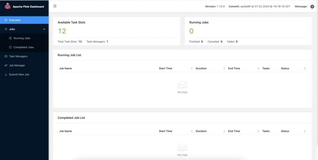
As mentioned earlier, Flink job is packed into docker-compose next way: We are using pyflink/playgrounds:1.10.0 image, which is the official docker image for Flink. You need to be careful with your volumes, in our case is ./examples:/opt/examples. On port localhost:8088 you will have Flink Dashboard with available data and stats about all your Flink jobs.
version: '2.1'
services:
  jobmanager:
    image: pyflink/playgrounds:1.10.0
    volumes:
      - ./examples:/opt/examples
    hostname: "jobmanager"
    expose:
      - "6123"
    ports:
      - "8088:8088"
    command: jobmanager
    environment:
      - JOB_MANAGER_RPC_ADDRESS=jobmanager
  taskmanager:
    image: pyflink/playgrounds:1.10.0
    volumes:
      - ./examples:/opt/examples
    expose:
      - "6121"
      - "6122"
    depends_on:
      - jobmanager
    command: taskmanager
    links:
      - jobmanager:jobmanager
    environment:
      - JOB_MANAGER_RPC_ADDRESS=jobmanager
Dockerfile:
FROM flink:1.10.0-scala_2.11

RUN set -ex; \
  apt-get update; \
  apt-get -y install python3; \
  apt-get -y install python3-pip; \
  apt-get -y install python3-dev; \
  ln -s /usr/bin/python3 /usr/bin/python; \
  ln -s /usr/bin/pip3 /usr/bin/pip


RUN set -ex; \
  apt-get update; \
  python -m pip install --upgrade pip; \
  pip install apache-flink; \
  pip install kafka-python

ARG FLINK_VERSION=1.10.0

RUN wget -P /opt/flink/lib/ https://repo.maven.apache.org/maven2/org/apache/flink/flink-json/${FLINK_VERSION}/flink-json-${FLINK_VERSION}.jar; \
    wget -P /opt/flink/lib/ https://repo.maven.apache.org/maven2/org/apache/flink/flink-csv/${FLINK_VERSION}/flink-csv-${FLINK_VERSION}.jar; \
    wget -P /opt/flink/lib/ https://repo.maven.apache.org/maven2/org/apache/flink/flink-sql-connector-elasticsearch6_2.11/${FLINK_VERSION}/flink-sql-connector-elasticsearch6_2.11-${FLINK_VERSION}.jar; \
    wget -P /opt/flink/lib/ https://repo.maven.apache.org/maven2/org/apache/flink/flink-sql-connector-kafka_2.11/${FLINK_VERSION}/flink-sql-connector-kafka_2.11-${FLINK_VERSION}.jar; \

# Create data folders
    mkdir -p /opt/data; \
    echo "taskmanager.memory.jvm-metaspace.size: 512m" >> /opt/flink/conf/flink-conf.yaml; \
    echo "rest.port: 8088" >> /opt/flink/conf/flink-conf.yaml;


WORKDIR /opt/flink/
Step 7: Run everything
To run everything from below we need three additional commands:
Run python script to generate dummy data:
python dummy_data_generator.pyBuild and run docker:
docker-compose up --buildAfter a while, you’ll be able to go to localhost:8088 and see the next page:
In the end, add PyFlink job to job manager:
docker-compose exec jobmanager ./bin/flink run -py /opt/examples/queries/app.pyYou’ll see a “job submitted” message which indicates you have a running job viewable on Flink Dashboard. Now you need to wait a little bit, depending on the time you choose as a window. After those moments passed, you can take a look at output_file.csv and see your results.
Step 8: Extra step
In case you want the output to ElasticSearch (running in Docker too), you can just add code-block from below to your docker-compose:
elasticsearch:
    image: docker.elastic.co/elasticsearch/elasticsearch-oss:6.3.1
    environment:
      - cluster.name=docker-cluster
      - bootstrap.memory_lock=true
      - "ES_JAVA_OPTS=-Xms512m -Xmx512m"
      - discovery.type=single-node
    ports:
      - "9200:9200"
      - "9300:9300"
    ulimits:
      memlock:
        soft: -1
        hard: -1
      nofile:
        soft: 65536
        hard: 65536
And in app.py change the sink function with the code block below:
def register_transactions_es_sink(st_env):
    st_env.connect(Elasticsearch()
                   .version("6")
                   .host("0.0.0.0", 9200, "http")
                   .index("transactions-supermarket-case")
                   .document_type("usage")) \
        .with_schema(Schema()
                     .field("customer", DataTypes.STRING())
                     .field("count_transactions", DataTypes.STRING())
                     .field("total_online_payment_amount", DataTypes.DOUBLE())
                     .field('total_in_store_payment_amount', DataTypes.DOUBLE())
                     .field("lon", DataTypes.FLOAT())
                     .field("lat", DataTypes.FLOAT())
                     .field('last_transaction_time', DataTypes.STRING())
                     ) \
        .with_format(Json().derive_schema()).in_upsert_mode().register_table_sink("sink_elasticsearch")
I hope this can be a great lead for you to start with your own streaming service and build on top of them. Flink was a little late on stage compared to Apache Storm and Apache Spark, but lately, the community of Flink is growing really fast which ensures fast-paced development of new features and everything you need to do is to use it. Also, it will give you a true streaming experience.
In today’s industries, it is not enough only to stream data with basic filters and joins, but to include machine learning models to help you better recognize real patterns, create recommendation systems, forecast your spent and profit, cluster your customers, etc. In consideration of that, the next blog on Apache Flink will include one of the mentioned machine learning methods in combination with streaming.
Meanwhile, take a look to a blogpost about recommendations in Covid time and stay tuned, because there will be more of this within our blog.
Featured Photo by Marta Wave from Pexels