How to boost online sales this holiday season with a personalized shopping experience
The holiday season is the most crucial period for retailers. Besides high sales volume, it is also an opportunity to…
Read moreThings Solver: Agentic AI + Customer 360 + Data Management
26. 01. 2019.

When dealing with anomalies in the data, there are lots of challenges that should be solved. We’ve already had a couple of articles regarding this topic, and if you haven’t already read it, I suggest you to take a look at this one, aaand this one, from my fellow colleague Miloš. In this post, I’m going to talk about one of my biggest favourites amongst anomaly detection algorithms. It is simple, superfast and efficient, with low memory requirement and linear time complexity. I’m not going to talk about the usage, since I stumbled upon a great article on Towards Data Science (check it out: Outlier Detection with Isolation Forest). The idea is to share my impressions, and to inspire you to try it out, and give me your feedback about it.
As you can pre-assume, the Isolation Forest is an ensemble-based method. And if you’re familiar with how the Random Forest works (I know you are, we all love it!), there is no doubt that you’ll quickly master the Isolation Forest algorithm. So, how does it work?
One thing that should be clarified prior to the algorithm explanation is the concept of the “instance isolation”. While most of other algorithms are trying to model the normal behaviour, to learn the profile patterns, this algorithm tries to separate the anomalous instance from the rest of the data (thus the term “isolation”). The easier it is to isolate the instance, the higher the chances are it is anomalous. Like the authors from this paper suggest, most existing model-based approaches to anomaly detection construct a profile of normal instances, then identify instances that do not conform to the normal profile as anomalies. What is the problem with that? Well, defining the normal behaviour. The boundaries of normal behaviour. In most cases, it is too expensive and time-consuming to label the data, and get the information of normal and anomalous behaviour. And that is when the creativity steps out and takes place on the stage. To create a simple, but borderline ingenuity (okay, I’m a little bit biased here :D).
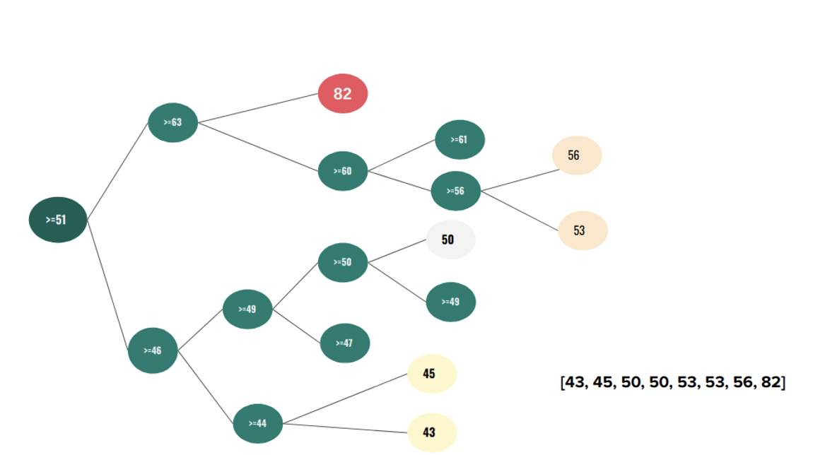
So, basically, Isolation Forest (iForest) works by building an ensemble of trees, called Isolation trees (iTrees), for a given dataset. A particular iTree is built upon a feature, by performing the partitioning. If we have a feature with a given data range, the first step of the algorithm is to randomly select a split value out of the available range of values. When the split value is chosen, the partitioning starts – each instance with a feature value lower than the split value is routed in the one side of the tree, while each instance with a feature value higher or equal than the split value is routed in the opposite side of the tree. In the second step, another random split value is selected, out of the available range of values for each side of the tree. This is recursively done until all instances are placed into terminal nodes (leaves), or some of the criteria set in the input parameters is met. The simplified process of building a tree is depicted below.
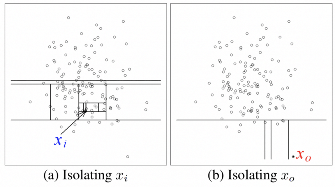
The idea is simple – if the instance is easily isolated (meaning there were fewer steps taken in order to place it into a terminal node), it has higher chances to be an anomaly. From the image that follows, it can be noticed that Xi instance from a dense area required many steps in order to be isolated, while the lonely Xo instance required far less.
So, in the iForest algorithm, the anomaly score is determined by the path length from the root node to the leaf in which the instance is placed. Since is it an ensemble, the average of all the path lengths for a given instance is taken. It can be induced that the average path length and anomaly score are inversely proportional – the shorter the path, the higher the anomaly score. In case I was totally confusing, I will just leave the official documentation here.
There are two main parameters – the number of trees, and the sub-sampling size. The sub-sampling size controls the size of the sample that will be used from model training, when partitioning is done. In the official documentation, the authors suggest that they have empirically found that optimal values for these parameters are 100 and 256, for number of trees and sub-sampling size, respectively.
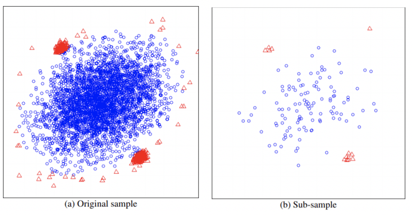
Now, there are two main problems that can be encountered when dealing with anomaly detection: swamping and masking. Swamping is a situation of wrongly identifying the normal instances as anomalous, which can happen when normal and anomalous instances are close to each other. Masking is the situation of wrongly identifying anomalous instances as normal, frequently happening when they are collectively situated in a dense area, so that they “conceal” their own presence. The sub-sampling in the iForest allows it to build a partial model that is resistant to these two effects. The next image shows how a subsampling could solve both problems easily. It can be noticed that sub-sampling cleared out the normal instances surrounding anomaly clusters, and reduced the size of anomalous clusters, which could lead to requiring more steps for isolation.
The scikit-learn implementation has some additional parameters like the maximum number of features to be considered, and contamination – the percent of anomalies that should be identified, which is quite nice. It basically works in such a way that a given percent of instances with the highest anomaly score is flagged as anomalous. It has a decision_function() which calculates the average anomaly score, and functions for fitting and predicting. And we haven’t gotten to the biggest forte of the algorithm yet! It can work both in supervised and unsupervised mode, which makes it a truly hidden hero of the machine learning realms. So, you can either feed it with the input data and labels, or only with the input data, it will crunch it and return the output.
In order to reduce a bias, let’s talk about drawbacks, since there are some of them. The first, and the most important one – it is not able to work with multivariate time series, which is one of the biggest problems we are facing in practice. Regarding the scikit-learn implementation, one thing that really bothers me is that it is not possible to get the particular decision for each iTree. Besides, it is also impossible to visualize the trees, and let’s be honest – people looove to see the picture. There is nothing they like more than a perfectly depicted algorithm they can interpret all by themselves. It could be really useful to see which feature caused the anomaly, and of which intensity. Another thing that concerns me here is – how will it behave with the features that are slightly deviant? I’m afraid that it can lead to the similar path lengths, and to the problem of masking (correct me if I’m wrong). Finally, I haven’t really tested it with the categorical data, but if someone has the experience with it, please drop me a line.
Regarding its nature, Isolation Forest shows enviable performances when working with high-dimensional or redundant data. It is pretty powerful when fitted in appropriate way and for problems that doesn’t require contextual anomaly detection (like time series, or spacial analysis). And as it is superfast, I really like to use it. I’ve tried it on the retail and on the telco data, and the results were pretty satisfying.
Anomaly detection is still one of the biggest problems analysts encounter when working with data. There is no doubt that there will be more algorithms for detecting anomalies in the data, with lots of improvements and capabilities. But the most important thing is not to neglect the significance and impact of anomalies on the results and decision making, because they represent a very sensitive problem and should be carefully approached and analysed. Keep that in mind. Cheers! [nz_icons icon=”icon-wink” animate=”false” size=”small” type=”circle” icon_color=”” background_color=”” border_color=”” /]

The holiday season is the most crucial period for retailers. Besides high sales volume, it is also an opportunity to…
Read more
The holiday season is the most crucial period for retailers. Besides high sales volume, it is also an opportunity to…
Read more
A closer look at analytics that matter You’ve trained your AI agent. It runs. It talks. It reacts. But does…
Read more
Imagine having a team of top chefs, but your fridge is packed with spoiled ingredients. No matter how talented they…
Read more