How to boost online sales this holiday season with a personalized shopping experience
The holiday season is the most crucial period for retailers. Besides high sales volume, it is also an opportunity to…
Read moreThings Solver: Agentic AI + Customer 360 + Data Management
16. 11. 2018.
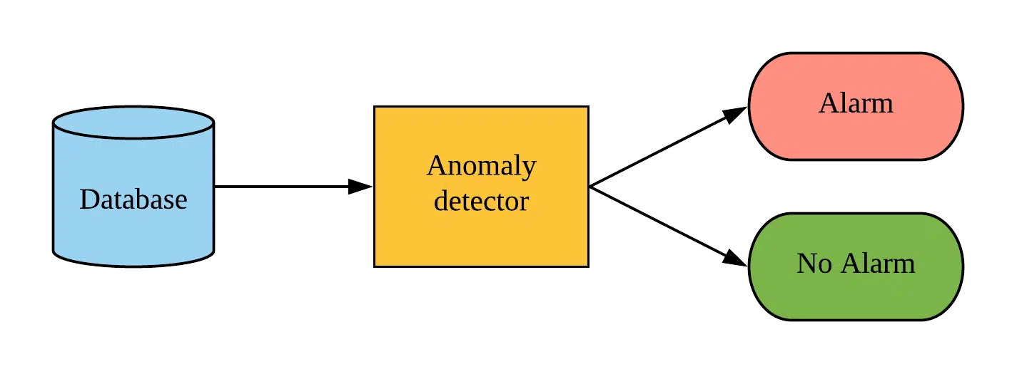
Let’s say you are tracking a large number of business-related or technical KPIs (that may have seasonality and noise). It is in your interest to automatically isolate a time window for a single KPI whose behavior deviates from normal behavior (contextual anomaly – for the definition refer to this post). When you have the problematic time window at hand you can further explore the values of that KPI. You can then link the anomaly to an event which caused the unexpected behavior. Most importantly, you can then act on the information.
To do the automatic time window isolation we need a time series anomaly detection machine learning model. The goal of this post is to introduce a probabilistic neural network (VAE) as a time series machine learning model and explore its use in the area of anomaly detection. As this post tries to reduce the math as much as possible, it does require some neural network and probability knowledge.
As Valentina mentioned in her post there are three different approaches to anomaly detection using machine learning based on the availability of labels:
Someone who has knowledge of the domain needs to assign labels manually. Therefore, acquiring precise and extensive labels is a time consuming and an expensive process. I’ve deliberately put unsupervised as the first approach, since it doesn’t require labels. It does, however, require that normal instances outnumber the abnormal ones. Not only do we require an unsupervised model, we also require it to be good at modeling non-linearities.

A model that has made the transition from complex data to tabular data is an Autoencoder(AE). Autoencoder consists of two parts – encoder and decoder. It tries to learn a smaller representation of its input (encoder) and then reconstruct its input from that smaller representation (decoder). An anomaly score is designed to correspond to the reconstruction error.
Autoencoder has a probabilistic sibling Variational Autoencoder(VAE), a Bayesian neural network. It tries not to reconstruct the original input, but the (chosen) distribution’s parameters of the output. An anomaly score is designed to correspond to an – anomaly probability. Choosing a distribution is a problem-dependent task and it can also be a research path. Now we delve into slightly more technical details.
Both AE and VAE use a sliding window of KPI values as an input. Model performance is mainly determined by the size of the sliding window.
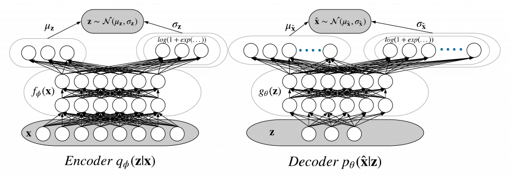
The smaller representation in the VAE context is called a latent variable and it has a prior distribution (chosen to be the Normal distribution). The encoder is its posterior distribution and the decoder is its likelihood distribution. Both of them are Normal distribution in our problem. A forward pass would be:
Variational Autoencoder as probabilistic neural network (also named a Bayesian neural network). It is also a type of a graphical model. An in-depth description of graphical models can be found in Chapter 8 of Christopher Bishop‘s Machine Learning and Pattern Recongnition.
A TensorFlow definition of the model:
class VAE(object):
    def __init__(self, kpi, z_dim=None, n_dim=None, hidden_layer_sz=None):
        """
        Args:
          z_dim : dimension of latent space.
          n_dim : dimension of input data.
        """
        if not z_dim or not n_dim:
            raise ValueError("You should set z_dim"
                             "(latent space) dimension and your input n_dim."
                             " \n            ")

        tf.reset_default_graph()

        def make_prior(code_size):
            loc = tf.zeros(code_size)
            scale = tf.ones(code_size)
            return tfd.MultivariateNormalDiag(loc, scale)

        self.z_dim = z_dim
        self.n_dim = n_dim
        self.kpi = kpi
        self.dense_size = hidden_layer_sz

        self.input = tf.placeholder(dtype=tf.float32,shape=[None, n_dim], name='KPI_data')
        self.batch_size = tf.placeholder(tf.int64, name="init_batch_size")

        # tf.data api
        dataset = tf.data.Dataset.from_tensor_slices(self.input).repeat() \
            .batch(self.batch_size)
        self.ite = dataset.make_initializable_iterator()
        self.x = self.ite.get_next()

        # Define the model.
        self.prior = make_prior(code_size=self.z_dim)
        x = tf.contrib.layers.flatten(self.x)
        x = tf.layers.dense(x, self.dense_size, tf.nn.relu)
        x = tf.layers.dense(x, self.dense_size, tf.nn.relu)
        loc = tf.layers.dense(x, self.z_dim)
        scale = tf.layers.dense(x, self.z_dim , tf.nn.softplus)
        self.posterior = tfd.MultivariateNormalDiag(loc, scale)
        self.code = self.posterior.sample()

        # Define the loss.
        x = self.code
        x = tf.layers.dense(x, self.dense_size, tf.nn.relu)
        x = tf.layers.dense(x, self.dense_size, tf.nn.relu)
        loc = tf.layers.dense(x, self.n_dim)
        scale = tf.layers.dense(x, self.n_dim , tf.nn.softplus)
        self.decoder = tfd.MultivariateNormalDiag(loc, scale)
        self.likelihood = self.decoder.log_prob(self.x)
        self.divergence = tf.contrib.distributions.kl_divergence(self.posterior, self.prior)
        self.elbo = tf.reduce_mean(self.likelihood - self.divergence)
        self._cost = -self.elbo

        self.saver = tf.train.Saver()
        self.sess = tf.Session()
def fit(self, Xs, learning_rate=0.001, num_epochs=10, batch_sz=200, verbose=True):

        self.optimize = tf.train.AdamOptimizer(learning_rate).minimize(self._cost)

        batches_per_epoch = int(np.ceil(len(Xs[0]) / batch_sz))
        print("\n")
        print("Training anomaly detector/dimensionalty reduction VAE for KPI",self.kpi)
        print("\n")
        print("There are",batches_per_epoch, "batches per epoch")
        start = timer()

        self.sess.run(tf.global_variables_initializer())

        for epoch in range(num_epochs):
            train_error = 0


            self.sess.run(
                self.ite.initializer,
                feed_dict={
                    self.input: Xs,
                    self.batch_size: batch_sz})

            for step in range(batches_per_epoch):
                _, loss = self.sess.run([self.optimize, self._cost])
                train_error += loss
                if step == (batches_per_epoch - 1):
                        mean_loss = train_error / batches_per_epoch
            if verbose:
                print(
                    "Epoch {:^6} Loss {:0.5f}"  .format(
                        epoch + 1, mean_loss))

            if train_error == np.nan:
                return False
        end = timer()
        print("\n")
        print("Training time {:0.2f} minutes".format((end - start) / (60)))
        return True
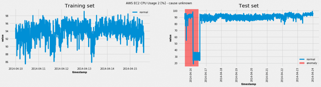
Using the model on one of the data sets from the Numenta Anomaly Benchmark(NAB):
In this case the model was able to achieve a true positive rate (TPR = 1.0) and a false positive rate (FPR = 0.07). For various anomaly probability thresholds we get a ROC curve:
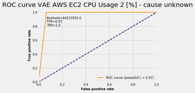
Choosing the threshold read from the ROC curve plot we get the following from the test set:
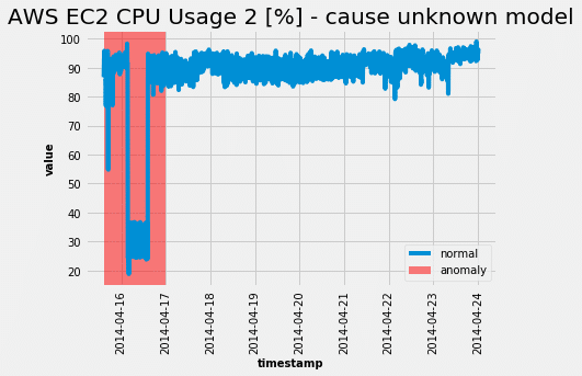
Just as the ROC curve suggested, the model was able to completely capture the abnormal behavior. Alas, as all neural network models are in need of hyperparameter tuning, this beast is no exception. However the only hyperparameter that can greatly affect the performance is the size of the sliding window.
I hope I was successful in introducing this fairly complex model in simple terms. I encourage you to try the model on other data sets available from here.
Keep on learning and things solving!

The holiday season is the most crucial period for retailers. Besides high sales volume, it is also an opportunity to…
Read more
The holiday season is the most crucial period for retailers. Besides high sales volume, it is also an opportunity to…
Read more
A closer look at analytics that matter You’ve trained your AI agent. It runs. It talks. It reacts. But does…
Read more
Imagine having a team of top chefs, but your fridge is packed with spoiled ingredients. No matter how talented they…
Read more